Python API
-
class
minepy.MINE(alpha=0.6, c=15, est="mic_approx")¶ Maximal Information-based Nonparametric Exploration.
Parameters: - alpha (float (0, 1.0] or >=4) – if alpha is in (0,1] then B will be max(n^alpha, 4) where n is the number of samples. If alpha is >=4 then alpha defines directly the B parameter. If alpha is higher than the number of samples (n) it will be limited to be n, so B = min(alpha, n).
- c (float (> 0)) – determines how many more clumps there will be than columns in every partition. Default value is 15, meaning that when trying to draw x grid lines on the x-axis, the algorithm will start with at most 15*x clumps.
- est (str ("mic_approx", "mic_e")) – estimator. With est=”mic_approx” the original MINE statistics will be computed, with est=”mic_e” the equicharacteristic matrix is is evaluated and the mic() and tic() methods will return MIC_e and TIC_e values respectively.
-
compute_score(x, y)¶ Computes the (equi)characteristic matrix (i.e. maximum normalized mutual information scores.
-
mic()¶ Returns the Maximal Information Coefficient (MIC or MIC_e).
-
mas()¶ Returns the Maximum Asymmetry Score (MAS).
-
mev()¶ Returns the Maximum Edge Value (MEV).
-
mcn(eps=0)¶ Returns the Minimum Cell Number (MCN) with eps >= 0.
-
mcn_general()¶ Returns the Minimum Cell Number (MCN) with eps = 1 - MIC.
-
gmic(p=-1)¶ Returns the Generalized Maximal Information Coefficient (GMIC).
-
tic(norm=False)¶ Returns the Total Information Coefficient (TIC or TIC_e). If norm==True TIC will be normalized in [0, 1].
-
get_score()¶ Returns the maximum normalized mutual information scores (i.e. the characteristic matrix M if est=”mic_approx”, the equicharacteristic matrix instead). M is a list of 1d numpy arrays where M[i][j] contains the score using a grid partitioning x-values into i+2 bins and y-values into j+2 bins.
-
computed()¶ Return True if the (equi)characteristic matrix) is computed.
Convenience functions
-
minepy.pstats(X, alpha=0.6, c=15, est="mic_approx")¶ Compute pairwise statistics (MIC and normalized TIC) between variables (convenience function).
For each statistic, the upper triangle of the matrix is stored by row (condensed matrix). If m is the number of variables, then for i < j < m, the statistic between (row) i and j is stored in k = m*i - i*(i+1)/2 - i - 1 + j. The length of the vectors is n = m*(m-1)/2.
Parameters: - X (2D array_like object) – An n-by-m array of n variables and m samples.
- alpha (float (0, 1.0] or >=4) – if alpha is in (0,1] then B will be max(n^alpha, 4) where n is the number of samples. If alpha is >=4 then alpha defines directly the B parameter. If alpha is higher than the number of samples (n) it will be limited to be n, so B = min(alpha, n).
- c (float (> 0)) – determines how many more clumps there will be than columns in every partition. Default value is 15, meaning that when trying to draw x grid lines on the x-axis, the algorithm will start with at most 15*x clumps.
- est (str ("mic_approx", "mic_e")) – estimator. With est=”mic_approx” the original MINE statistics will be computed, with est=”mic_e” the equicharacteristic matrix is is evaluated and MIC_e and TIC_e are returned.
Returns: - mic (1D ndarray) – the condensed MIC statistic matrix of length n*(n-1)/2.
- tic (1D ndarray) – the condensed normalized TIC statistic matrix of length n*(n-1)/2.
-
minepy.cstats(X, Y, alpha=0.6, c=15, est="mic_approx")¶ Compute statistics (MIC and normalized TIC) between each pair of the two collections of variables (convenience function).
If n and m are the number of variables in X and Y respectively, then the statistic between the (row) i (for X) and j (for Y) is stored in mic[i, j] and tic[i, j].
Parameters: - X (2D array_like object) – An n by m array of n variables and m samples.
- Y (2D array_like object) – An p by m array of p variables and m samples.
- alpha (float (0, 1.0] or >=4) – if alpha is in (0,1] then B will be max(n^alpha, 4) where n is the number of samples. If alpha is >=4 then alpha defines directly the B parameter. If alpha is higher than the number of samples (n) it will be limited to be n, so B = min(alpha, n).
- c (float (> 0)) – determines how many more clumps there will be than columns in every partition. Default value is 15, meaning that when trying to draw x grid lines on the x-axis, the algorithm will start with at most 15*x clumps.
- est (str ("mic_approx", "mic_e")) – estimator. With est=”mic_approx” the original MINE statistics will be computed, with est=”mic_e” the equicharacteristic matrix is is evaluated and MIC_e and TIC_e are returned.
Returns: - mic (2D ndarray) – the MIC statistic matrix (n x p).
- tic (2D ndarray) – the normalized TIC statistic matrix (n x p).
First Example
The example is located in examples/python_example.py.
import numpy as np
from minepy import MINE

def print_stats(mine):
    print "MIC", mine.mic()
    print "MAS", mine.mas()
    print "MEV", mine.mev()
    print "MCN (eps=0)", mine.mcn(0)
    print "MCN (eps=1-MIC)", mine.mcn_general()
    print "GMIC", mine.gmic()
    print "TIC", mine.tic()

x = np.linspace(0, 1, 1000)
y = np.sin(10 * np.pi * x) + x
mine = MINE(alpha=0.6, c=15, est="mic_approx")
mine.compute_score(x, y)

print "Without noise:"
print_stats(mine)
print

np.random.seed(0)
y +=np.random.uniform(-1, 1, x.shape[0]) # add some noise
mine.compute_score(x, y)

print "With noise:"
print_stats(mine)
Run the example:
$ python python_example.py
Without noise:
MIC 1.0
MAS 0.726071574374
MEV 1.0
MCN (eps=0) 4.58496250072
MCN (eps=1-MIC) 4.58496250072
GMIC 0.779360251901
TIC 67.6612295532

With noise:
MIC 0.505716693417
MAS 0.365399904262
MEV 0.505716693417
MCN (eps=0) 5.95419631039
MCN (eps=1-MIC) 3.80735492206
GMIC 0.359475501353
TIC 28.7498326953
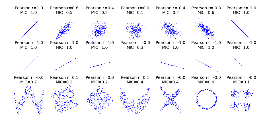
Second Example
The example is located in examples/relationships.py.
Warning
Requires the matplotlib library.
from __future__ import division
import numpy as np
import matplotlib.pyplot as plt
from minepy import MINE


rs = np.random.RandomState(seed=0)

def mysubplot(x, y, numRows, numCols, plotNum,
              xlim=(-4, 4), ylim=(-4, 4)):

    r = np.around(np.corrcoef(x, y)[0, 1], 1)
    mine = MINE(alpha=0.6, c=15, est="mic_approx")
    mine.compute_score(x, y)
    mic = np.around(mine.mic(), 1)
    ax = plt.subplot(numRows, numCols, plotNum,
                     xlim=xlim, ylim=ylim)
    ax.set_title('Pearson r=%.1f\nMIC=%.1f' % (r, mic),fontsize=10)
    ax.set_frame_on(False)
    ax.axes.get_xaxis().set_visible(False)
    ax.axes.get_yaxis().set_visible(False)
    ax.plot(x, y, ',')
    ax.set_xticks([])
    ax.set_yticks([])
    return ax

def rotation(xy, t):
    return np.dot(xy, [[np.cos(t), -np.sin(t)], [np.sin(t), np.cos(t)]])

def mvnormal(n=1000):
    cors = [1.0, 0.8, 0.4, 0.0, -0.4, -0.8, -1.0]
    for i, cor in enumerate(cors):
        cov = [[1, cor],[cor, 1]]
        xy = rs.multivariate_normal([0, 0], cov, n)
        mysubplot(xy[:, 0], xy[:, 1], 3, 7, i+1)

def rotnormal(n=1000):
    ts = [0, np.pi/12, np.pi/6, np.pi/4, np.pi/2-np.pi/6,
          np.pi/2-np.pi/12, np.pi/2]
    cov = [[1, 1],[1, 1]]
    xy = rs.multivariate_normal([0, 0], cov, n)
    for i, t in enumerate(ts):
        xy_r = rotation(xy, t)
        mysubplot(xy_r[:, 0], xy_r[:, 1], 3, 7, i+8)

def others(n=1000):
    x = rs.uniform(-1, 1, n)
    y = 4*(x**2-0.5)**2 + rs.uniform(-1, 1, n)/3
    mysubplot(x, y, 3, 7, 15, (-1, 1), (-1/3, 1+1/3))

    y = rs.uniform(-1, 1, n)
    xy = np.concatenate((x.reshape(-1, 1), y.reshape(-1, 1)), axis=1)
    xy = rotation(xy, -np.pi/8)
    lim = np.sqrt(2+np.sqrt(2)) / np.sqrt(2)
    mysubplot(xy[:, 0], xy[:, 1], 3, 7, 16, (-lim, lim), (-lim, lim))

    xy = rotation(xy, -np.pi/8)
    lim = np.sqrt(2)
    mysubplot(xy[:, 0], xy[:, 1], 3, 7, 17, (-lim, lim), (-lim, lim))

    y = 2*x**2 + rs.uniform(-1, 1, n)
    mysubplot(x, y, 3, 7, 18, (-1, 1), (-1, 3))

    y = (x**2 + rs.uniform(0, 0.5, n)) * \
        np.array([-1, 1])[rs.random_integers(0, 1, size=n)]
    mysubplot(x, y, 3, 7, 19, (-1.5, 1.5), (-1.5, 1.5))

    y = np.cos(x * np.pi) + rs.uniform(0, 1/8, n)
    x = np.sin(x * np.pi) + rs.uniform(0, 1/8, n)
    mysubplot(x, y, 3, 7, 20, (-1.5, 1.5), (-1.5, 1.5))

    xy1 = np.random.multivariate_normal([3, 3], [[1, 0], [0, 1]], int(n/4))
    xy2 = np.random.multivariate_normal([-3, 3], [[1, 0], [0, 1]], int(n/4))
    xy3 = np.random.multivariate_normal([-3, -3], [[1, 0], [0, 1]], int(n/4))
    xy4 = np.random.multivariate_normal([3, -3], [[1, 0], [0, 1]], int(n/4))
    xy = np.concatenate((xy1, xy2, xy3, xy4), axis=0)
    mysubplot(xy[:, 0], xy[:, 1], 3, 7, 21, (-7, 7), (-7, 7))

plt.figure(facecolor='white')
mvnormal(n=800)
rotnormal(n=200)
others(n=800)
plt.tight_layout()
plt.show()
Convenience functions example
The example is located in examples/python_conv_example.py.
import numpy as np
from minepy import pstats, cstats
import time

np.random.seed(0)

# build the X matrix, 8 variables, 320 samples
X = np.random.rand(8, 320)

# build the Y matrix, 4 variables, 320 samples
Y = np.random.rand(4, 320)

# compute pairwise statistics MIC_e and normalized TIC_e between samples in X,
# B=9, c=5
mic_p, tic_p =  pstats(X, alpha=9, c=5, est="mic_e")

# compute statistics between each pair of samples in X and Y
mic_c, tic_c =  cstats(X, Y, alpha=9, c=5, est="mic_e")

print "normalized TIC_e (X):"
print tic_p
print "MIC_e (X vs. Y):"
print mic_c
$ python python_conv_example.py
normalized TIC_e (X):
[ 0.01517556  0.00859132  0.00562575  0.01082706  0.01367201  0.0196697
  0.00947777  0.01273158  0.011291    0.01455822  0.0072817   0.01187837
  0.01595135  0.00902464  0.00974791  0.00952264  0.01806944  0.01064587
  0.00808622  0.01075486  0.00943122  0.01116569  0.01380142  0.01590193
  0.02159243  0.01450488  0.01347701  0.01036625]
MIC_e (X vs. Y):
[[ 0.0175473   0.01102385  0.01489008  0.02957048]
 [ 0.01294067  0.02682975  0.02743612  0.02224291]
 [ 0.01613576  0.0175808   0.01633154  0.02633199]
 [ 0.02090252  0.01680651  0.01735732  0.02186021]
 [ 0.01350926  0.01002233  0.02128154  0.02036634]
 [ 0.01459962  0.020248    0.0319421   0.01782455]
 [ 0.01186273  0.0291112   0.01577821  0.01970322]
 [ 0.012531    0.02071883  0.01536824  0.03312674]]